Introduction
This part of the learning activity focuses on learning objective #2:
- Demonstrate an understanding of key statistical concepts: hypothesis testing, \(p\) values, confidence intervals and power
Hypothesis tests are the key statistical tests employed in most clinical trials.
You are likely to have come across most of these terms before, and, hopefully, the previous section has helped you to recall and refine some of you statistical intuitions.
Important definitions
- Null hypothesis
the statistical hypothesis that there is no (important) difference between experimental treatment and control in relation to the primary endpoint
- Sampling distribution
is the distribution of expected results expected assuming a particular hypothesis about the effect size is true (e.g. the null hypothesis), all the assumptions associated with the statistical model are true, and the trial is conducted as planned.
- Type I error (\(\alpha\))
is the pre-test probability of rejecting the null hypothesis when the null hypothesis is true. It is usually set at 0.05.
- Type II error (\(\beta\))
\(\beta\) is the pre-test probability of accepting the null hypothesis when the alternative hypothesis is true.
- Power \((1-\beta)\)
is the pre-study probability that the study will produce a statistically significant result for a given sample size and postulated effect size
- \(p\) value
a measure of the compatibility of the observed data with the data that would be expected if the null hypothesis was true when all other statistical and methodological assumptions are met
- Confidence interval
is the range of effect sizes that is considered more compatible with the observed data assuming the statistical and methodological assumptions of the study are met. A 95% confidence interval provides the range of values for which a test of an effect size within the range against the observed data would provide a \(p\) value \(> 0.05\).
Interpretation
Standard hypothesis tests are set up in such a way that if the observed data falls into the \(\alpha\) region, then observing such a result is more likely if the alternative hypothesis is true compared to if the null hypothesis is true. This is an important aspect of the justification for rejecting the null hypothesis and accepting the alternative hypothesis.
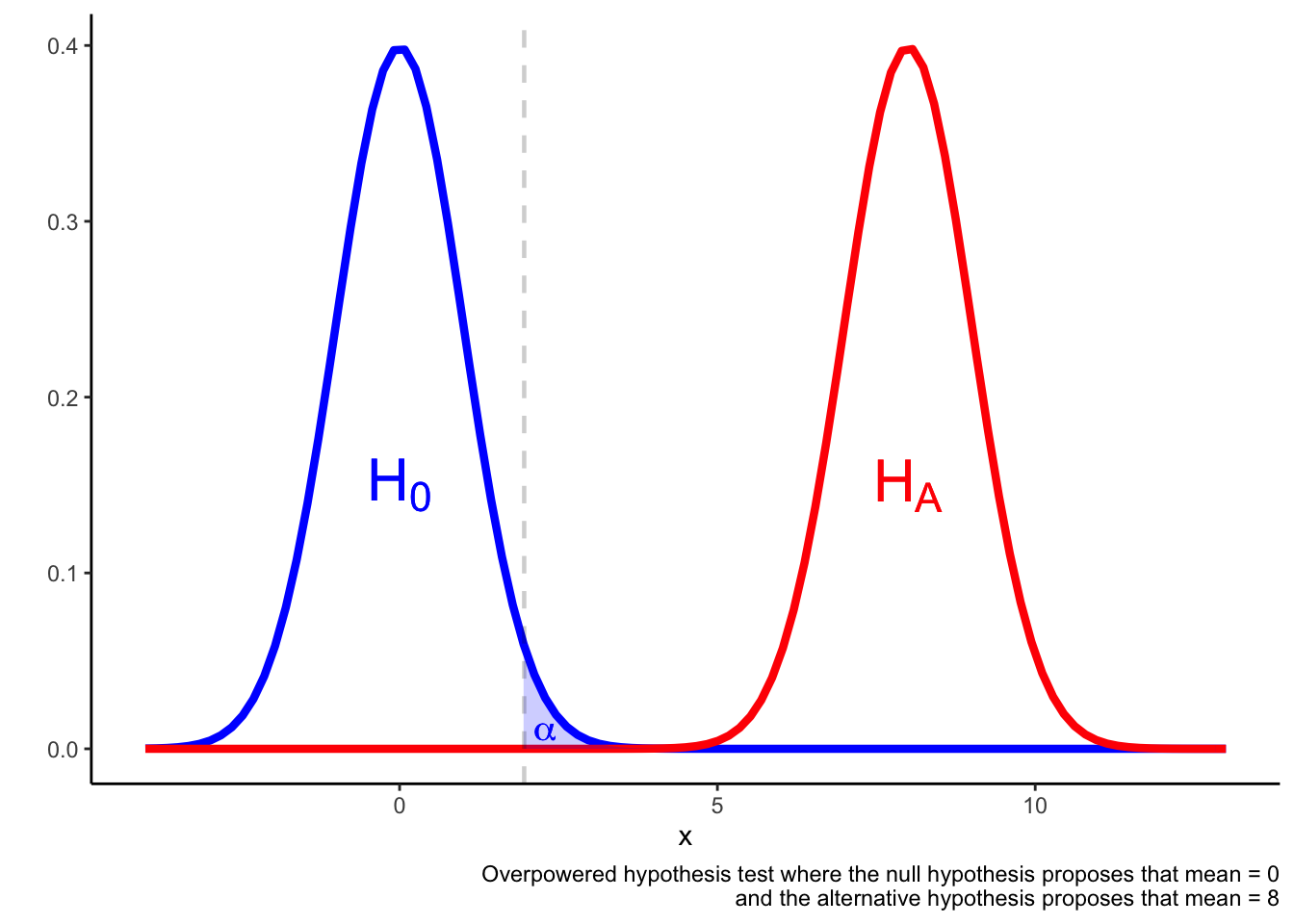
Assuming the outcome is a continuous variable that is normally distributed, the following figure illustrates the set-up of a hypothesis test.

A hypothesis test is set up to avoid Type I and Type II errors. Type I errors occur when you reject the null hypothesis when the null hypothesis is true. Type II errors occur when you fail to reject the null hypothesis despite the null hypothesis being false.
One way to avoid type I and type II errors is to ensure \(\alpha\) is sufficiently small and the statistical test is adequately powered. A suitable rule of thumb is that \(\beta \approx 0.2\) (which is equivalent to a power of 80%).
In an overpowered test, it may be the case that a result in the \(\alpha\) region is more likely if the null hypothesis is true rather than if the alternative hypothesis is true.
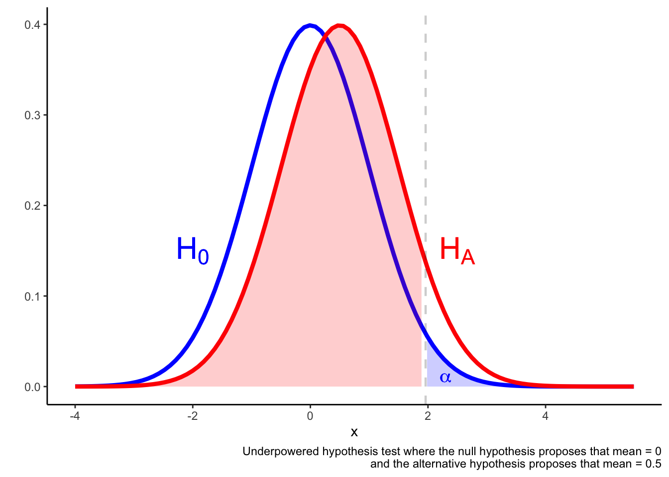
In an underpowered test, it may be the case that a result in the \(\alpha\) region is not much more likely if the alternative hypothesis is true compared if the alternative hypothesis is true. The result falling in the \(\alpha\) region is not a reliable indicator that he null is false.
Setting up a hypothesis test
The power of the test is considered before collecting any data, but after the research question and statistical test have been identified. The information you need will depend on the specific statistical test, but here are some general principles. The statistical power of the test depends on:
Sample size: the larger the sample, the higher the power.
You also need to think about loss to follow-up, drop-outs and non-adherence to the study.
Estimated effect size: this is the effect size you are trying to detect (perhaps the difference between two means). The smaller the estimated effect size, the lower the power
This might be determined by existing evidence, or it might be the “minimally clinically important difference”.
Variability in the sample: the more variability in the sample, the lower the power of the test
Predetermined \(\alpha\), \(\beta\): standard values are \(\alpha = 0.05\), \(\beta = 0.2\), but if you change these, you will change the power of the test (obviously, I hope)
Interpreting results of tests with different power
The following 2 X 2 table provides some guidance on the interpretation of hypothesis tests that are adequately powered and those that are underpowered.
| Statistically significant result | Non-statistically significant result | |
|---|---|---|
| Adequately powered test | Reject the null. Accept the alternative hypothesis | The test failed to reject the null. Either the null is true or the effect size is smaller than was tested |
| Underpowered test | Provisionally accept the alternative hypothesis | Underdetermined result. The test is unable to detect effect sizes that might be important. |
Worked example
Consider the primary statistical results for the CURE study (The CURE Investigators 2001).
CURE Study PICO (The CURE Investigators 2001)
P: Patients within 24 hours of admission with acute coronary syndrome; average age approx. 64; multiple cardiovascular risk factors; patients with risk of bleeding excluded
I: Clopidogrel in addition to aspirin and other aspects of standard care
C: Aspirin and other aspects of standard care
O: Primary endpoint: cardiovascular death, nonfatal MI or stroke; important safety endpoint: major bleed
The scientific hypothesis that is under test in CURE is that there is no difference when patients with acute coronary syndrome (ACS) are given clopidogrel plus aspirin when compared to aspirin alone.
The statistical hypothesis tested in the study has additional details. A test statistic is chosen, in this case the test statistic is the relative risk of the primary endpoint (cardiovascular death, nonfatal MI or stroke). Notice that different measures could be chosen at this point—e.g. hazard rate, absolute risk—and different items could be included in the relative risk measure—e.g. overall mortality.
Further details include the size of the CURE study, the expected effect size that the trial will be powered to test. All of these details specify the statistical hypothesis that is under test in CURE.
Statistical results for the primary endpoint are provided in the abstract:
The first primary outcome …occurred in 9.3 percent of the patients in the clopidogrel group and 11.4 percent of the patients in the placebo group (relative risk with clopidogrel as compared with placebo, 0.80; 95 percent confidence interval, 0.72 to 0.90; \(P < 0.001\)).
How should we interpret these results?
CURE Study: Set up & Results
The null hypothesis is that there is no difference in outcome between participants who received clopidogrel plus aspirin compared to the participants who received aspirin alone.
The null hypothesis provides a statistical model that can be tested by the study. An important part of the statistical model for the null hypothesis is that the true relative risk for the primary endpoint is 1 (i.e. no difference in primary endpoint event rates in participants that received clopidogrel and aspirin compared to aspirin alone)
The \(p\) value for the primary endpoint is low (\(p < 0.001\)); the observed data (relative risk 0.80) would be unexpected if the null hypothesis and associated statistical model was true
The \(p\) is below our arbitrary cut-off for “rejecting the null hypothesis”
Inference: clopidogrel in addition to aspirin reduces the risk of event(s) within the primary endpoint (in the participants in the trial, treated under the conditions of the trial)
The 95% confidence interval is a measure of the precision of the trial; the size of CURE means that the 95% confidence interval is quite small: 0.72–0.90
Interpretation
The \(p\) value is a measure of the compatibility of the observed data with a statistical model that assumes the null hypothesis is true and all other statistical and methodological assumptions are met
The lower the \(p\) value, the more incompatible the observed data is with the statistical model
\(p < 0.05\) is an arbitrary cut-off for statistical significance
\(p < 0.05\) is considered to license the inference that the null hypothesis is false (assuming the other assumptions in the model are met)
Randomized trials are designed to provide a rigorous test of the primary endpoint; statistically significant results on other endpoints in the study are often less reliable
Confidence intervals are a measure of the precision of the statistical result (assuming the statistical and methodological assumptions are met)
If a \(p\) value \(< 0.05\) is observed one of the following has occurred:
The null hypothesis is false
The statistical model, or one of the assumptions involved in specifying the statistical model, is false
A chance event has occurred
xkcd.com has some apt comics: see \(p\) values and significant.
Greenland et al. (2016) provides a helpful discussion of common misinterpretations of the \(p\) value. For instance, it is very tempting to interpret the \(p\) value as a measure of the probability that the null hypothesis is true (and such an interpretation is often implied in elementary texts on statistical hypotheses). But this is not the correct interpretation. The probability of the null hypothesis being true or false is influenced by a host of factors that are not directly considered in the calculation of the \(p\) value. One important factor is the prior probability of the null and alternative hypotheses. If the prior probability of the alternative hypothesis is very low, a statistical result that suggests the rejection of the null and acceptance of the alternative won’t necessarily raise that probability very high. See Ioannidis (2005) for further details.
Summary
Some people find statistics challenging. Like any other challenging area, the more you read about it and use it, the more it starts to fit together.
If some of the discussion above is confusing, here are some general principles to keep in mind:
- The most-often used cut-off for \(p\) values used in clinical research is 0.05.
- If the \(p\) value is \(< 0.05\), the result will be considered statistically significant
- A statistically significant result for the primary endpoint of a trial is more trustworthy than statistically significant results on secondary endpoints or subgroups—the trial was set up the test the primary endpoint.
- Once you have determined that the primary endpoint of trial was statistically significant, the next question is to determine whether the magnitude of the effect is clinically significant—this relies on clinical reasoning and thinking through whether the observed difference on the endpoint is of importance.
Tasks
Focusing on the primary endpoint of the study, identify the PICO, null hypothesis and the statistical result for each of the studies for which links to abstracts are provided below. Based on the information available to you, what inference does the study support?
- Zinman et al. (2015) Empagliflozin, Cardiovascular Outcomes, and Mortality in Type 2 Diabetes
- Rosenstock et al. (2018) Effect of ertugliflozin on glucose control, body weight, blood pressure and bone density in type 2 diabetes mellitus inadequately controlled on metformin monotherapy (VERTIS MET)
- SEARCH Collaborative Group (2010) Intensive lowering of LDL cholesterol with 80 mg versus 20 mg simvastatin daily in 12 064 survivors of myocardial infarction: a double-blind randomised trial
References
Greenland, Sander, Stephen J. Senn, Kenneth J. Rothman, John B. Carlin, Charles Poole, Steven N. Goodman, and Douglas G. Altman. 2016. “Statistical Tests , P-values , Confidence Intervals , and Power : A Guide to Misinterpretations.” The American Statistician 15 (053): 1–31. https://doi.org/10.1007/s10654-016-0149-3.
Ioannidis, John P A. 2005. “Why Most Published Research Findings Are False.” PLoS Medicine 2 (8): e124. https://doi.org/10.1371/journal.pmed.0020124.
Rosenstock, Julio, Juan Frias, Dénes Páll, Bernard Charbonnel, Raluca Pascu, Didier Saur, Amanda Darekar, et al. 2018. “Effect of ertugliflozin on glucose control, body weight, blood pressure and bone density in type 2 diabetes mellitus inadequately controlled on metformin monotherapy (VERTIS MET).” Diabetes, Obesity and Metabolism 20 (3): 520–29. https://doi.org/10.1111/dom.13103.
SEARCH Collaborative Group. 2010. “Intensive lowering of LDL cholesterol with 80 mg versus 20 mg simvastatin daily in 12 064 survivors of myocardial infarction: A double-blind randomised trial.” The Lancet 376 (10): 1658–69. https://doi.org/10.1016/S0140-6736(13)61970-4.
The CURE Investigators. 2001. “Effects of clopidogrel in addition to aspirin in patients with acute coronary syndromes without ST-segment elevation.” New England Journal of Medicine 345 (7): 494–502.
Zinman, Bernard, Christoph Wanner, John M. Lachin, David Fitchett, Erich Bluhmki, Stefan Hantel, Michaela Mattheus, et al. 2015. “Empagliflozin, Cardiovascular Outcomes, and Mortality in Type 2 Diabetes.” New England Journal of Medicine 373 (22): 2117–28. https://doi.org/10.1056/NEJMoa1504720.