Developing intuitions about statistical inference

Most people have some idea of what \(p\) values, confidence intervals and power mean. But their intuitions frequently miss some of the important aspects of these concepts—or worse—get them completely muddled (Greenland et al. 2016). There are a couple of reasons for this. Partly, it is because the concepts themselves can be complex, and partly it is because of the way these concepts are taught. Key statistical concepts are often taught in a way that simplifies the complexity.

Understanding the logic of statistical inference is a good first step to understanding and applying the key statistical concepts.

Statistical approaches seek to reduce the influence of random error on inference.

Fair coin

Consider tosses of a fair coin. You don’t expect to observe 5 ‘heads’ (\(H\)) every time that you toss a fair coin 10 times. The variation that occurs between what we observe and what we would expect given our assumptions about tossing a fair coin is called random error.

Here is the outcome of an experiment that consists in tossing a fair coin 10 times. The outcome is provided using the statistical program R—the process is equivalent to tossing a fair coin 10 times where 1 is considered \(H\) and 0 is considered \(T\).

##  [1] 0 1 0 1 1 0 1 1 1 0

In this series of tosses, there were 6 \(H\) and 4 \(T\).

If we run the same code a second time, we get:

##  [1] 0 1 1 0 0 0 0 1 0 0

This time we see 3 \(H\) and 7 \(T\). There is no surprise about this variation and there is also no doubt that our coin is “fair”—this is stipulated in the code that produced the outcome. What we are observing is random error.

We expect the number of \(H\) in any series of 10 tosses to bounce around. Sometimes it might be 5, 3, 8, 2, 6,… etc.

A histogram represents how many times we observed specific outcomes from the 10 coin toss experiment. Here is a histogram of the set of results we observed when we repeat the 10 coin toss experiment 10 times. The result below provides the number of \(H\) in each 10-toss experiment.

##  [1] 5 8 5 5 7 5 7 4 7 4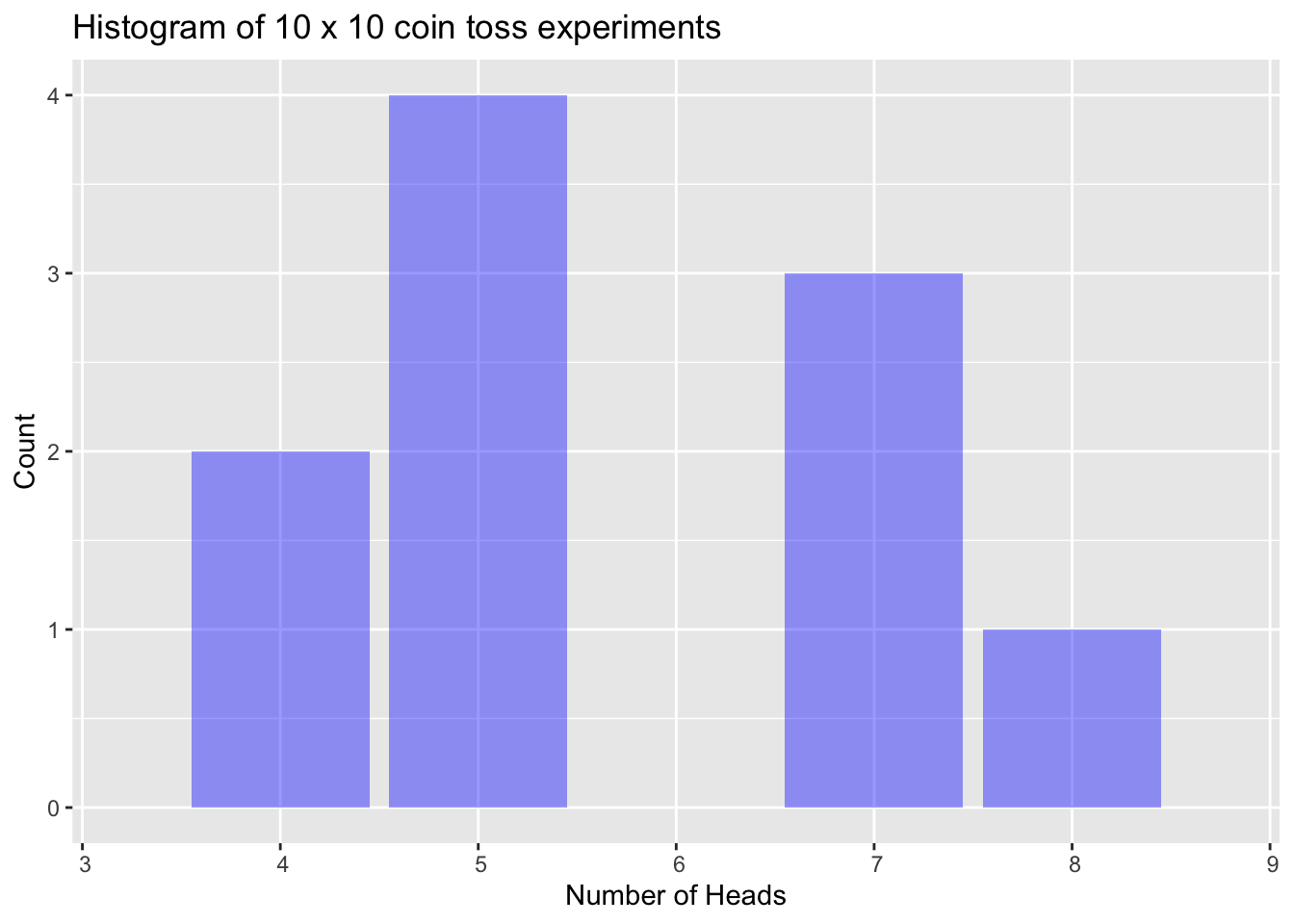

The mean number of \(H\) in this series was 5.7. This is higher than we would expect given that we know the coin is fair, but again, we need to be mindful that the overall number of coin tosses is quite low.

The effects of random error are more significant when the number of coin tosses, or participants, is low. The larger the number of coin tossing experiments we conduct the more confident we can be that the mean number of \(H\) across all experiments will be close to 5.

Here is a histogram for the results we observe if we repeat the 10 coin toss experiment 10,000 times.

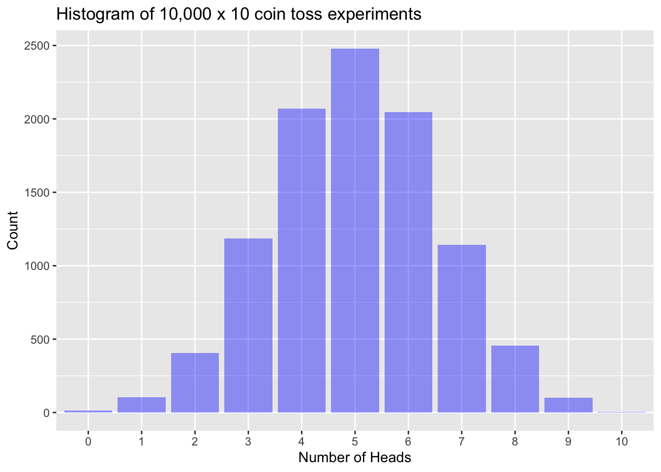
With this large number of 10 coin toss experiments we start to see some regularity in the data. While there a a number of 10 coin toss experiments that provided 0 \(H\) or 10 \(H\), more experiments provided an outcome of 5 \(H\) or close to 5 \(H\) compared to \(< 2\) or \(> 8\). The mean number of \(H\) across all of these experiments was 4.998, very close to what we expect given the coin is fair.

There are a couple of important lessons from this:

1. Random error can make it hard to make inference from small samples of data. We knew the coin was fair, but from a small number of 10 coin toss experiments we will see a range of results that are compatible with a the coin not being fair.
2. Increasing the number of repetitions provided mean results much closer to what we expect given the coin is fair. Notice that we can model the expected results of repetitions of the 10 coin toss experiment without doing any experiments—our expectations can be defined mathematically based on assumptions we make about the probability of \(H\) and the nature of the coin tossing experiment (i.e. that each toss is independent and the result of each toss depends on the probability of \(H\)).

These are the building blocks for statistical inference. #1 emphasises the importance of ensuring a sufficient sample size to reduce the impact of random error. And #2 provides a statistical model against which we can compare observations of actual experiments.

Coin of unknown bias

How could we test whether a coin of unknown bias was fair?

The strategy used by the classical statistical methods employed in most clinical trials is provided below. While I refer to some statistical concepts here, they are more formally introduced in the next section.

1. Consider what outcomes we would expect if the coin was fair. This is called the null hypothesis. If the coin was fair and we conducted many repetitions of the 10 coin toss experiment, we would expect results like those seen in the experiment conducted above: a wide range of results—0 \(H\) to 10 \(H\)—but with many more results clustering around 5 \(H\); we also expect a mean result of approximately 5. This expectation, and the assumptions that go along with this expectation, provides a statistical model that we can use to inform our inferences.
2. Conduct repetitions of the 10 coin toss experiment with the coin of unknown bias.
3. Use what we know about the statistical model—i.e. the expected distribution of results if the coin was fair—, and considerations regarding the kind of difference that we will consider far enough away from fair to consider important, to determine how many repetitions of the 10 coin toss experiment we would need to do for our results to be reliable. For example, we might not be too worried about a coin that was biased in favour of \(H\) such that the probability of \(H\) was 0.50002—but if we were, we would need a very large number of repetitions. This is a consideration of study power.
4. Compare the mean observed result of the repetitions of the 10 coin toss experiments with the coin of unknown bias with what we would expect if the coin was fair.
5. If the observed mean of the repetitions of the 10 coin toss experiment is considerably larger or smaller than 5, then the study provides some evidence that the coin is not fair.
6. The probability of observing a result more extreme than the one we did can be calculated using the statistical model assuming the null hypothesis—this is the \(p\) value.

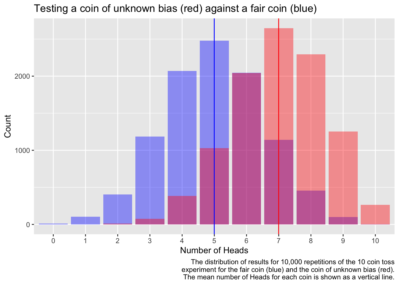
The mean number of \(H\) for the fair coin was 4.998 and for the coin of unknown bias was 6.9982. What do you think the probability of \(H\) is for the coin of unknown bias?

References

Greenland, Sander, Stephen J. Senn, Kenneth J. Rothman, John B. Carlin, Charles Poole, Steven N. Goodman, and Douglas G. Altman. 2016. “Statistical Tests , P-values , Confidence Intervals , and Power : A Guide to Misinterpretations.” The American Statistician 15 (053): 1–31. https://doi.org/10.1007/s10654-016-0149-3.