Assumptions about the data?

Despite the MAQ being a relatively simple survey, determining how we should interpret the data is not straightforward!

You could focus on each item and the different type of non-adherence it probes. It is common, for example, to interpret Q1 and Q2 as probing non-intentional non-adherence and Q3 and Q4 as probing intentional non-adherence. In this situation you could interpret the results of the MAQ as nominal data identifying different categories of non-adherence. (NB. you can’t do this with the data in example1.csv because you only have the total MAQ score).

Alternatively, you can focus on the overall MAQ score, which for each participant will be one of [0,1,2,3,4]. Now we have the question of whether this data is ordinal or discrete? Take care to understand the difference between these two assessments.

If the data are ordinal, we are not making any assumptions regarding the interval between scores. A score of 4 is higher than 3, just as a score of 2 is higher than 1—there is no claim that the difference between these scores is the same. If the data are ordinal, it makes sense to talk of medians, modes and interquartile ranges, but not means and standard deviations. We need to use non-parametric statistical analyses for ordinal data.

If the data are discrete we are claiming that the score is a measure and that the interval between the scores is the same. If the data are discrete, we can talk of means and standard deviations. If we decide to compare groups using mean MAQ, and we believe these means to be approximately normally distributed, we can use parametric statistical tests.

People will differ in their views regarding whether MAQ scores should be interpreted as ordinal or discrete. Given the MAQ has been so widely used, one of the things that can help you here is how the data has been treated in the past. MAQ data has frequently been treated as discrete data and mean MAQ has frequently been used to measure adherence in interventional studies and in studies assessing the association between the MAQ and other measures of medication taking behaviour.

In what follows we are going to treat the MAQ score as a discrete measure and use mean MAQ to compare the groups. We are also going to assume that mean MAQ is approximately normally distributed. (Later we will modify these assumptions and see if we get a different result).

Choice of statistical test

Given the assumptions we have made about the data we can use a t-test to compare the groups.

Two more decisions before we can do the analysis.

• Should we use a paired or unpaired t-test?
• Should we use a one-sided or two-sided test?

The first is a straightforward determination of the kinds of groups that we have. Since we have randomized allocation, we have two independent groups: we use the unpaired t-test. (A paired t-test is used when you are comparing linked results; e.g. a before-and-after test in the same individual).

The choice between a one-sided and two-sided test depends on the kind of hypothesis you are testing. Is your hypothesis that the groups are different? Or is your hypothesis that one group will have better adherence than the other?—i.e., Is your question non-directional or directional? In this case the hypothesis we wish to test is whether the group that received the intervention has improved adherence. For this reason we will use a one-sided test.

Analysis

example1.csv provides the data from the study. The dataset includes three columns: “baseline”, which provides the MAQ score at baseline, “end”, which provides the MAQ score at the end of the study (3 months) and “group”, which indicates whether the participant is in the intervention group, “I”, or the control group, “C”.

df <- read.csv(file = "csv/example1.csv", header = TRUE)  # reads the csv file into R for analysis

head(df)  # prints first lines of the dataframe

##   baseline end group
## 1        1   1     I
## 2        3   1     I
## 3        0   1     I
## 4        1   2     I
## 5        1   2     I
## 6        2   0     I

summary(df)  # print a summary of the dataset

##     baseline          end           group          
##  Min.   :0.000   Min.   :0.000   Length:120        
##  1st Qu.:1.000   1st Qu.:0.000   Class :character  
##  Median :2.000   Median :1.000   Mode  :character  
##  Mean   :1.625   Mean   :1.125                     
##  3rd Qu.:2.000   3rd Qu.:2.000                     
##  Max.   :4.000   Max.   :3.000

It often helps to summarise the data and plot it to get a picture of what is going on. I am not going to ask you to do this in the assignment.

# The following is to get the data into a form that we can plot. There are
# multiple ways of doing this, and they change over time. A helpful set of
# packages is provided within the `tidyverse` (https://www.tidyverse.org). The
# following is provided for completeness.

library(ggplot2)
library(reshape2)
library(plyr)

df_melt <- melt(df, id.vars = "group", measure.vars = c("baseline", "end"))


# a function to calculate the standard error:
se <- function(x) sqrt(var(x)/length(x))

# df_sum <- ddply(df_melt, c(df_melt$group,df_melt$variable), summarise, N =
# length(df_melt$value), mean = mean(df_melt$value), se = sd(df_melt$value) )

df_sum <- ddply(df_melt, .(group, variable), summarise, N = length(value), mean = mean(value),
    se = se(value))

df_sum  # provides a helpful summary of the data

##   group variable  N      mean        se
## 1     C baseline 60 1.6333333 0.1405531
## 2     C      end 60 1.4833333 0.1268739
## 3     I baseline 60 1.6166667 0.1387834
## 4     I      end 60 0.7666667 0.0990539

p3 <- ggplot(df_sum, aes(x = df_sum$variable, y = df_sum$mean, fill = df_sum$group)) +
    geom_bar(position = position_dodge(), stat = "identity") + geom_errorbar(aes(ymin = df_sum$mean -
    df_sum$se, ymax = df_sum$mean + df_sum$se), width = 0.2, size = 0.2, position = position_dodge(0.9)) +
    xlab("Time") + ylab("Mean MAQ") + labs(caption = "Mean MAQ plotted over time in the control and intervention group. Error bars are standard error.") +
    scale_fill_discrete(name = "Group", labels = c("Control", "Intervention")) +
    theme_minimal()

p3  #print the plot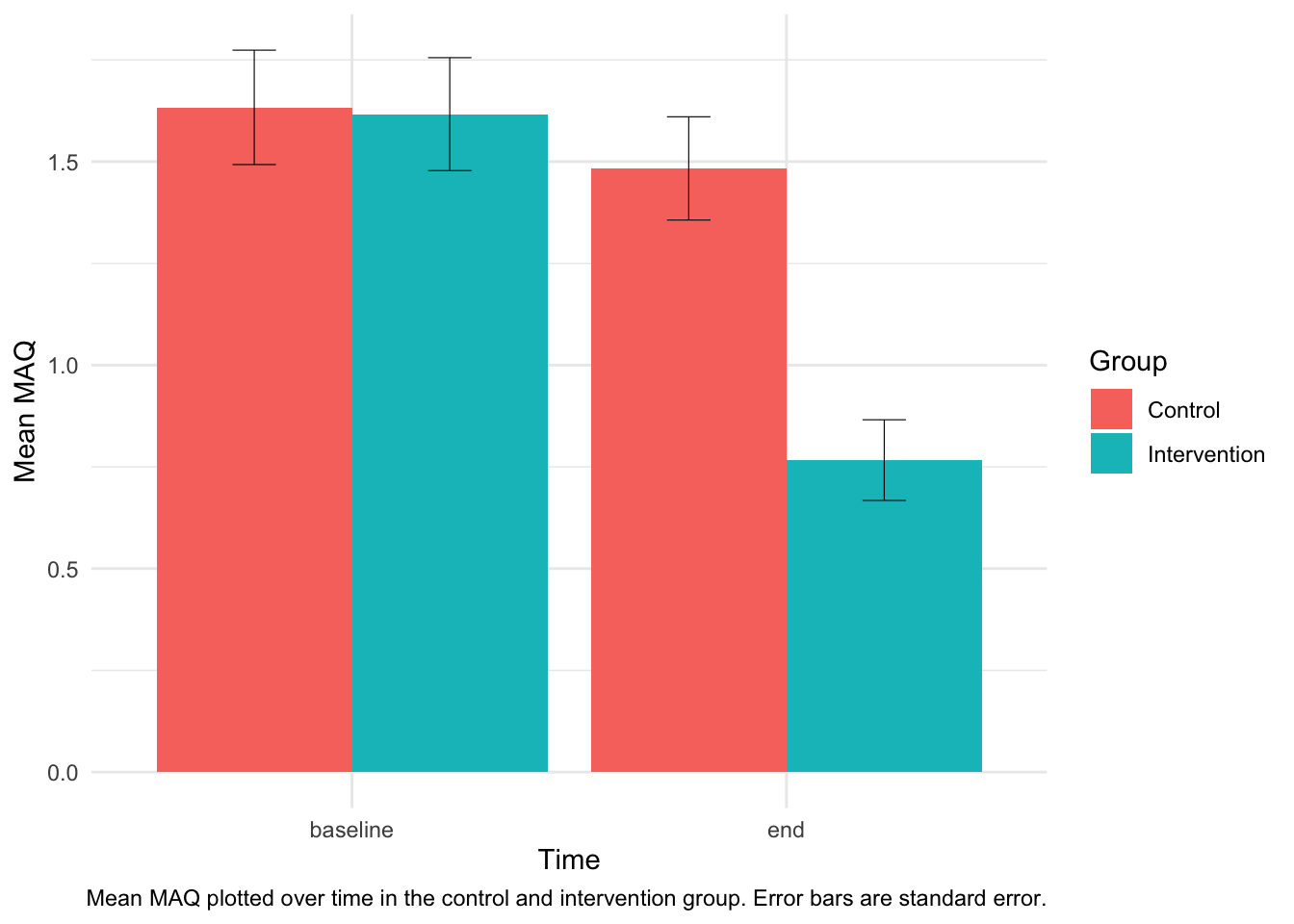

The plot shows that there appears to be an improvement in mean MAQ in the intervention group, but also that there is significant variability in the data.

Now we can do the t-test. The function in R is t.test()—see the documentation online here. You want to read the documentation of the test so that you know what you need to give the test and what it is doing to the data. It can take a while to get used to reading these documents, but they are very helpful. The documentation here is the same as the documentation you can call within R itself.

There are a couple of steps illustrated below:

1. Split the data into the intervention group and the control group
2. Conduct a two sided t-test on the baseline data to see if the groups were similar at the start of the study
3. Conduct a one sided t-test on the end data to see if the groups are different at the end of the study. This is the test of the primary hypothesis of the study.

# Split the dataframe up into those that received the intervention and those
# that did not
df_int <- subset(df, df$group == "I")
df_con <- subset(df, df$group == "C")

t.test(df_con$baseline, df_int$baseline, alternative = "two.sided")

## 
## 	Welch Two Sample t-test
## 
## data:  df_con$baseline and df_int$baseline
## t = 0.084378, df = 117.98, p-value = 0.9329
## alternative hypothesis: true difference in means is not equal to 0
## 95 percent confidence interval:
##  -0.3744867  0.4078200
## sample estimates:
## mean of x mean of y 
##  1.633333  1.616667

t.test(df_con$end, df_int$end, alternative = "greater")

## 
## 	Welch Two Sample t-test
## 
## data:  df_con$end and df_int$end
## t = 4.4524, df = 111.44, p-value = 1.013e-05
## alternative hypothesis: true difference in means is greater than 0
## 95 percent confidence interval:
##  0.4496889       Inf
## sample estimates:
## mean of x mean of y 
## 1.4833333 0.7666667

Interpretation

So what does this mean?

1. The groups were similar in terms of self-reported adherence at baseline
2. The group that received the intervention had a statistically significant improvement in self-reported adherence (i.e. observed as a lower mean MAQ). The mean MAQ in the intervention group was 0.77 and the mean MAQ in the control group was 1.48, \(p = 0.00001\).

Exercises

1. Notice that a “Welch Two Sample t-test” has been conducted. This is a more conservative test compared to the Student’s t-test. The difference is that Welch’s test does not assume the variance in the groups is equal. Re-run the test with the option, var.equal = TRUE, i.e. t.test(df_con$end, df_int$end, alternative = "greater", var.equal = TRUE) and note what happens.

2. Re-run the analysis, this time assuming the data is ordinal. What are the appropriate summary measures of the data? Which statistical test is appropriate? What result do you get if you run the test?

3. This time, use the MAQ data to dichotomise the group into “adherent” (MAQ = 0) and “non-adherent” (MAQ ≥ 1). What type of data is the MAQ data now? Assess whether the intervention increased the proportion participants characterised as adherent? What is the appropriate statistical test?

References

Nguyen, Thi-My-Uyen, Adam La Caze, and W Neil Cottrell. 2016. “Validated adherence scales used in a measurement-guided medication management approach to target and tailor a medication adherence intervention: a randomised controlled trial.” BMJ Open 6 (11): e013375. https://doi.org/10.1136/bmjopen-2016-013375.