Assess the association between two variables
Now we are going to assess correlation between two variables. We will continue to use the MAQ, and introduce a second scale that is used to assess an individual’s beliefs about their medicines.
Beliefs About Medicines Questionnaire (BMQ)
The BMQ-Specific comprises of 10 items which assess how the participant perceives the necessity of their medication (5 items) and their concerns regarding their medication (5 items). Each item is assessed on a 5-point Likert scale, where 1 = “strongly disagree,” 2 = “disagree,” 3 = “uncertain,” 4 = “agree” and 5 = “strongly agree.”
Therefore scores for BMQ-Necessity and BMQ-Concerns range from 5–25, with higher scores meaning the participant more strongly perceives their medicine is necessary, or more strongly perceives concerns regarding their medicine.
Again, the R code and csv files for dataset is provided so that you can run these analyses (or others) yourself.
Download the files here.
Research question
This time the research question is whether an individual’s beliefs about their medicines (as measured by the BMQ-Specific) is associated with their self-reported adherence (as measured by the MAQ).
Assumptions about the data?
Like we did for the first example, let’s start with the assumption that the MAQ data is discrete and that the mean MAQ is normally distributed.
We are going to make a similar assumption regarding the BMQ-Specific data. This could also be debated, but it is consistent with how these scales are used in the literature. Moreover, we tend to focus on the sum-scores of the two sub-scales: BMQ-necessity and BMQ-concerns. Given that we are adding the individual items within the sub-scale together, we are already assuming that these sub-scales provide interval data. We will also assume that mean scores for the two sub-scales are normally distributed.
Choice of statistical test
Given the assumptions we have made about the data we can assess the association between BMQ scores and MAQ scores using a Pearson correlation.
Analysis
example2.csv provides the data from the study.
The dataset includes eight columns: MAQ_1, MAQ_2, MAQ_3, MAQ_4 provide answers to each MAQ item (“yes” is coded as 1); MAQ provides the MAQ score. BMQ_N, BMQ_C and BMQ_Diff provide the BMQ-necessity, BMQ-concerns, and BMQ-differential (i.e. BMQ-necessity - BMQ-concerns).
df <- read.csv(file = "csv/example2.csv", header = TRUE)  # reads the csv file into R for analysis

head(df)  # prints first lines of the dataframe
## MAQ_1 MAQ_2 MAQ_3 MAQ_4 MAQ BMQ_N BMQ_C BMQ_Diff
## 1 0 0 0 1 1 20 13 7
## 2 1 1 0 0 2 19 12 7
## 3 0 0 1 0 1 17 13 4
## 4 1 0 0 0 1 23 12 11
## 5 0 0 0 1 1 18 16 2
## 6 0 0 0 0 0 23 15 8summary(df) # print a summary of the dataset## MAQ_1 MAQ_2 MAQ_3 MAQ_4
## Min. :0.0000 Min. :0.0000 Min. :0.0000 Min. :0.0000
## 1st Qu.:0.0000 1st Qu.:0.0000 1st Qu.:0.0000 1st Qu.:0.0000
## Median :1.0000 Median :0.0000 Median :0.0000 Median :0.0000
## Mean :0.5833 Mean :0.2667 Mean :0.1833 Mean :0.1833
## 3rd Qu.:1.0000 3rd Qu.:1.0000 3rd Qu.:0.0000 3rd Qu.:0.0000
## Max. :1.0000 Max. :1.0000 Max. :1.0000 Max. :1.0000
## MAQ BMQ_N BMQ_C BMQ_Diff
## Min. :0.000 Min. : 5.00 Min. : 5.00 Min. :-5.000
## 1st Qu.:1.000 1st Qu.:17.00 1st Qu.:10.00 1st Qu.: 3.000
## Median :1.000 Median :20.00 Median :12.00 Median : 7.000
## Mean :1.217 Mean :19.27 Mean :12.68 Mean : 6.592
## 3rd Qu.:2.000 3rd Qu.:22.00 3rd Qu.:15.00 3rd Qu.:10.000
## Max. :4.000 Max. :25.00 Max. :25.00 Max. :19.000Let’s plot the data. Scatterplots are good for observing possible associations between two variables.
p2 <- plot(df$BMQ_N, df$MAQ, pch = 19, ylab = "MAQ", xlab = "BMQ-necessity")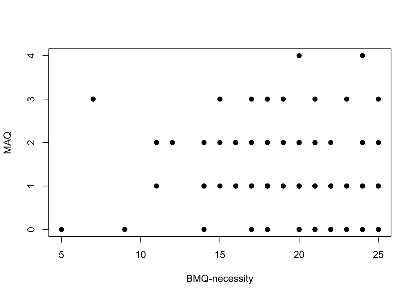
p3 <- plot(df$BMQ_C, df$MAQ, pch = 19, ylab = "MAQ", xlab = "BMQ-concerns")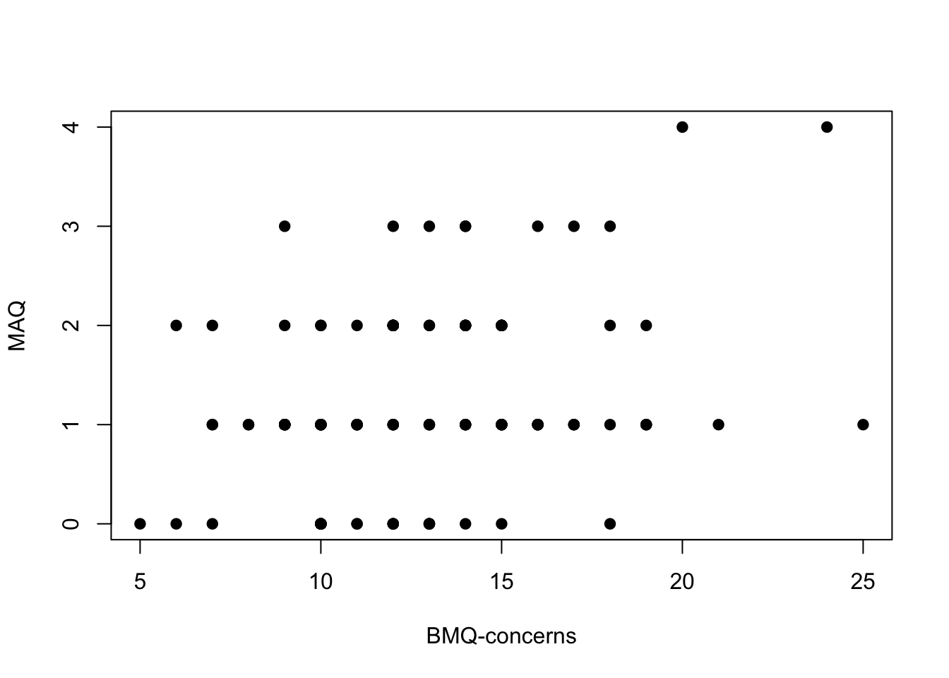
p4 <- plot(df$BMQ_Diff, df$MAQ, pch = 19, ylab = "MAQ", xlab = "BMQ-differential")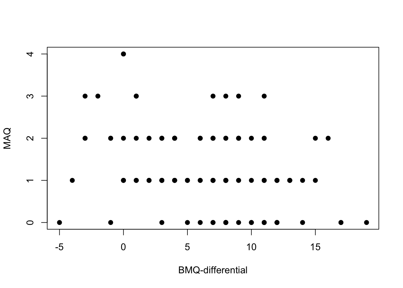
p5 <- plot(df$BMQ_N, df$BMQ_C, pch = 19, ylab = "BMQ-concerns", xlab = "BMQ-necessity")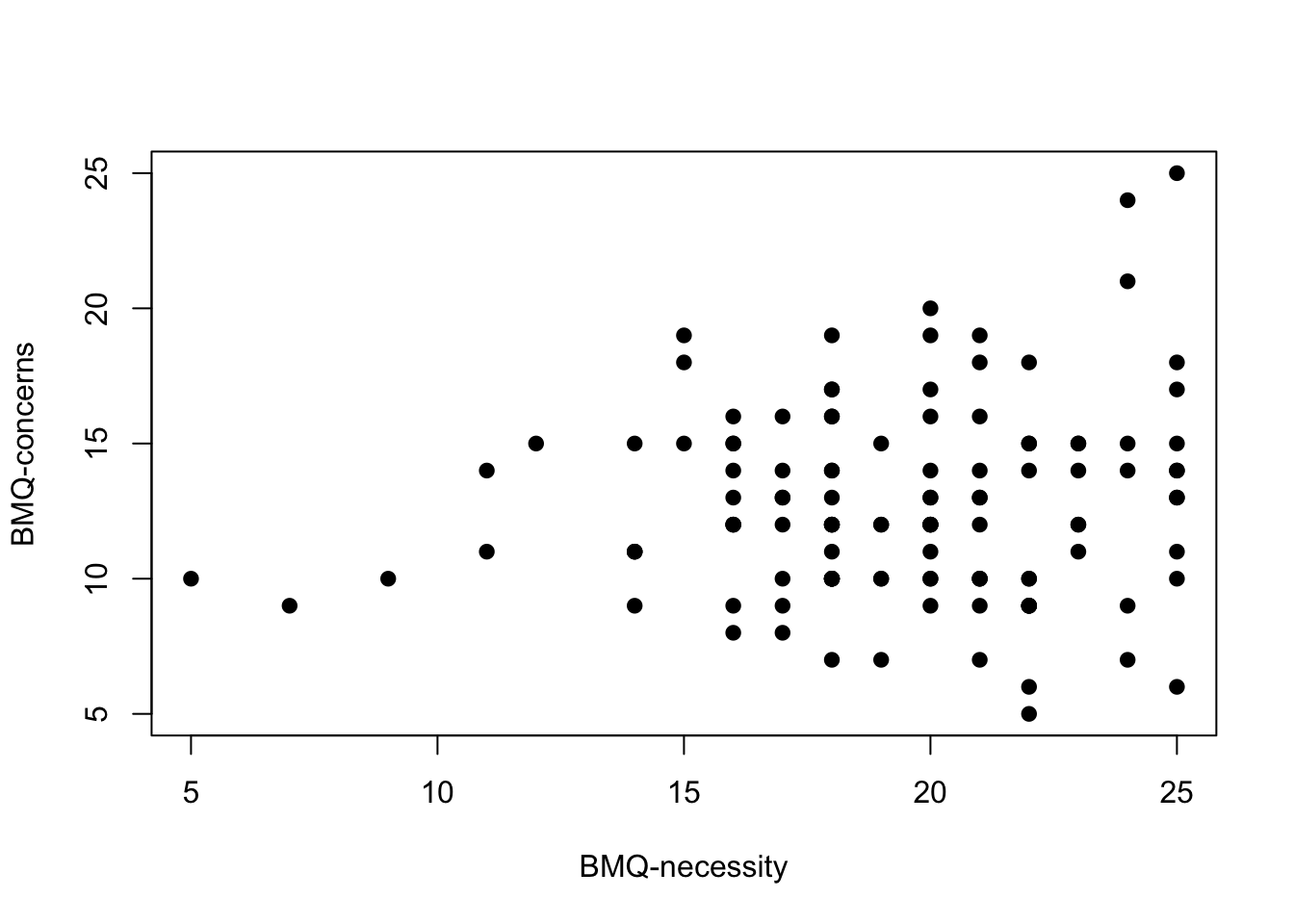
The first thing that is obvious in these plots is the effect of MAQ being discrete data with relatively few options. This makes it a little difficult to see any relationships.
If you squint a little you might see some relationships. Perhaps the clearest relationship is one we are not assessing: the relationship between BMQ-necessity and BMQ-concerns. There is an absence of people with low necessity scores and high concerns scores. It is worth noting, however, that there were relatively few participants with low necessity scores.
The two methods for assessing correlations in R are cor() and cor.test(). The first gives you the correlations (but doesn’t perform any tests), the second gives you the correlations and performs a test against the null hypothesis of no correlation.
Read the documentation!—cor, cor.test.
df_maq <- df[, c("BMQ_N", "BMQ_C", "BMQ_Diff", "MAQ")]

cor(df_maq, method = "pearson")
## BMQ_N BMQ_C BMQ_Diff MAQ
## BMQ_N 1.0000000 0.1262681 0.6860675 -0.1237816
## BMQ_C 0.1262681 1.0000000 -0.6350863 0.3166274
## BMQ_Diff 0.6860675 -0.6350863 1.0000000 -0.3286026
## MAQ -0.1237816 0.3166274 -0.3286026 1.0000000cor.test(df$BMQ_N, df$MAQ, method = "pearson")##
## Pearson's product-moment correlation
##
## data: df$BMQ_N and df$MAQ
## t = -1.355, df = 118, p-value = 0.178
## alternative hypothesis: true correlation is not equal to 0
## 95 percent confidence interval:
## -0.29644579 0.05671811
## sample estimates:
## cor
## -0.1237816cor.test(df$BMQ_C, df$MAQ, method = "pearson")##
## Pearson's product-moment correlation
##
## data: df$BMQ_C and df$MAQ
## t = 3.626, df = 118, p-value = 0.0004262
## alternative hypothesis: true correlation is not equal to 0
## 95 percent confidence interval:
## 0.1456523 0.4692382
## sample estimates:
## cor
## 0.3166274cor.test(df$BMQ_Diff, df$MAQ, method = "pearson")##
## Pearson's product-moment correlation
##
## data: df$BMQ_Diff and df$MAQ
## t = -3.7794, df = 118, p-value = 0.000248
## alternative hypothesis: true correlation is not equal to 0
## 95 percent confidence interval:
## -0.4795961 -0.1587091
## sample estimates:
## cor
## -0.3286026Interpretation
According to this test:
- There is a statistically significant correlation between:
- BMQ-concerns and MAQ score, Pearsons correlation 0.317, p = 0.0004, and
- BMQ-differential and MAQ score, Pearsons correlation -0.329, p = 0.0002
- There was no statistically significant correlation between BMQ-necessity and MAQ
Increased concerns regarding medications seems to reduce medication adherence. The larger the BMQ-differential (BMQ-necessity - BMQ-concerns) the better an individual’s adherence as measured by the MAQ score.
While the correlation is statistically significant, it is not a particularly strong correlation. Correlation varies from -1 to 1, with -1 demonstrating a perfect linear inverse correlation (as \(x\) increases, \(y\) decreases), 0 meaning the variables are independent and 1 demonstrating a perfect linear correlation (as \(x\) increases, \(y\) increases).
Exercises
- Re-run the analysis, this time assuming the data is ordinal. What are the appropriate summary measures of the data? Which statistical test is appropriate? What result do you get if you run the test?
- Develop your data manipulation skills in R. Divide the participants in
example2.csvin to those with low and high BMQ Necessity beliefs. (i) Assign participants with an BMQ_N score below the median, “LN,” to represent a low BMQ_N score (less than the median) and, “HN,” to represent a high BMQ_N score (greater than or equal to the median); (ii) identify participants who are identified by the MAQ as intentionally nonadherent (i.e. participants who answered “yes” to MAQ_Q3 or MAQ_Q4), and (iii) present a 2 x 2 table of participants grouped by low/high BMQ_N score and yes/no “intentional nonadherence.” Suggested tools:as.factor(),ifelse(),table().